C3.2 Curve Sketching
Geometric Applications of the Derivatives
increasing
f'(x)>0
concave up
f"(x)>0
f'(x)>0
concave up
f"(x)>0
increasing
f'(x)>0
concave down
f"(x)<0
f'(x)>0
concave down
f"(x)<0
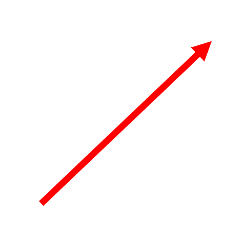
increasing
f'(x)>0
no concavity
f"(x)=0
f'(x)>0
no concavity
f"(x)=0
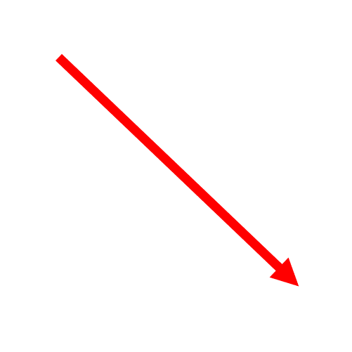
decreasing
f'(x)<0
concave up
f"(x)>0
f'(x)<0
concave up
f"(x)>0
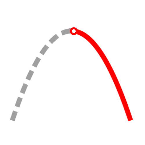
decreasing
f'(x)<0
concave down
f"(x)<0
f'(x)<0
concave down
f"(x)<0
decreasing
f'(x)<0
no concavity
f"(x)=0
f'(x)<0
no concavity
f"(x)=0
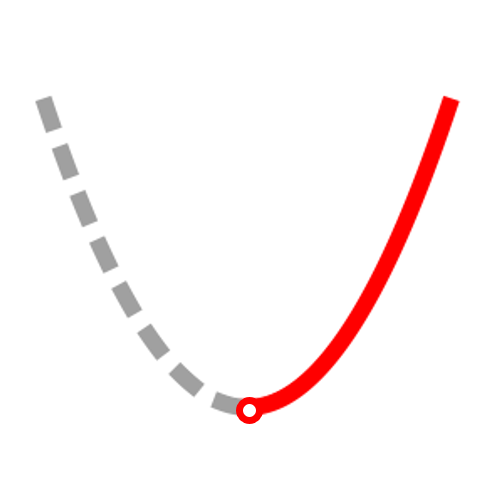
stationary point
f'(x)=0
concave up
f"(x)>0
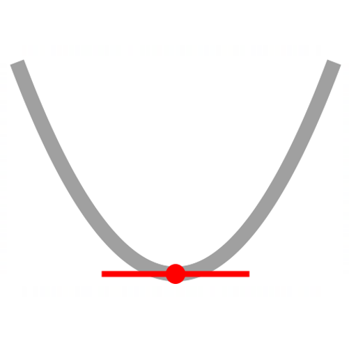
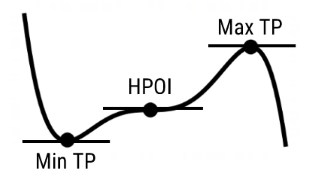
minimum TP
f'(x)=0
concave up
f"(x)>0
minimum TP
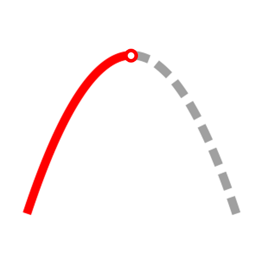
stationary point
f'(x)=0
concave down
f"(x)<0
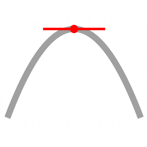
maxiumum TP
f'(x)=0
concave down
f"(x)<0
maxiumum TP
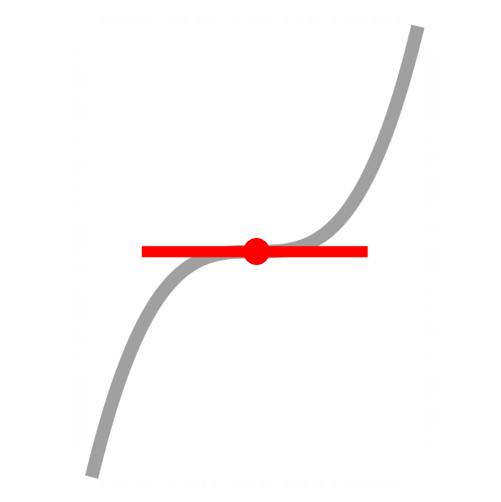
stationary point
f'(x)=0
change of concavity
f"(x)=0
horzontal POI
f'(x)=0
change of concavity
f"(x)=0
horzontal POI
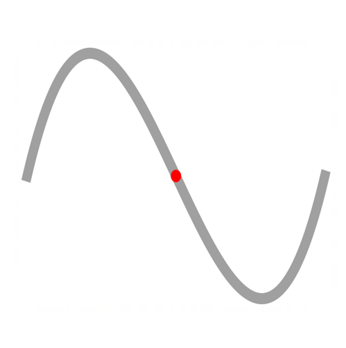
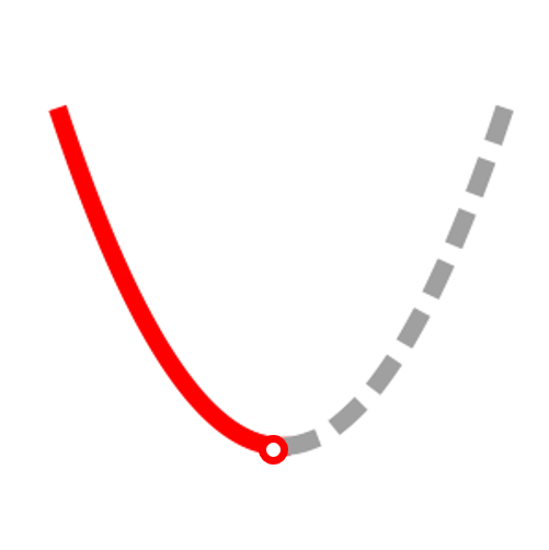
decreasing
f'(x)<0
change of concavity
f"(x)=0
point of inflection
f'(x)<0
change of concavity
f"(x)=0
point of inflection
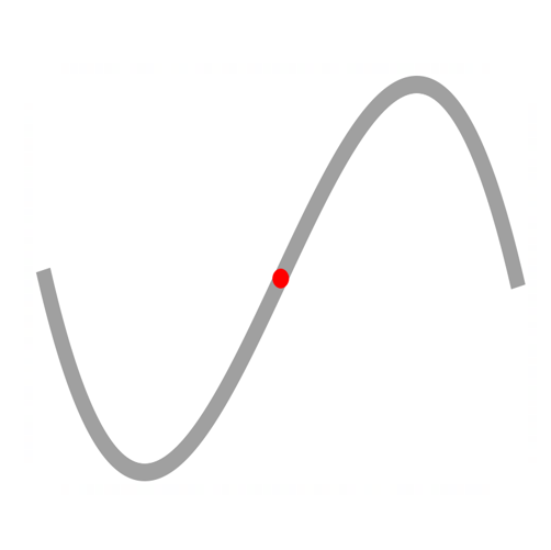
increasing
f'(x)>0
change of concavity
f"(x)=0
point of inflection
f'(x)>0
change of concavity
f"(x)=0
point of inflection
stationary point
f'(x)=0
change of concavity
f"(x)=0
horzontal POI
f'(x)=0
change of concavity
f"(x)=0
horzontal POI
Key Features of the Derivatives
- calculates the coordinates of points on graph
- solving \( f(x) = 0 \) finds the x-intercept(s) of the graph
- calculates the gradient of a graph at a point
- solving \( f'(x) = 0 \) finds the x-coordinate(s) of stationary point(s) on a graph
- calculates the concavity of a graph at a point
- solving \( f''(x) = 0 \) finds possible points of inflection on a graph (must be tested).
- Only look for points of inflection if the question specifically asks for them.
Suggested Steps for Curve Sketching
Step ❶ : Find \(f'(x)\) and, if possible, \(f''(x)\) - (Find the 1st and 2nd Derivatives)
Step ❷ : Set \(f'(x) = 0\) and solve for x - (Locate SP's)
- Sub the x-coordinate into f(x) to find the y-cordinate of the SP.
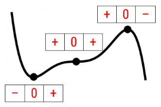
Step ❸ : Determine the nature of stationary points that have been located.
- First Derivative Test - (tests the slope either side of the SP)
- Substitute the x-coordinates of points either side of the SP into \(f'(x) \)
- A sign change of (-)(0)(+) indicates a minimum turning point.
- A sign change of (+)(0)(-) indicates a maximum turning point.
- No sign change [(+)(0)(+) or (-)(0)(-)] indicates a horizontal point of inflection.
- Second Derivative Test - (tests the concavity at SP)
- Substitute the x-coordinate of SP into \(f''(x) \).
- If the result is \(f''(x) > 0\), the curve is concave up and the SP is a minimum turning point.
- If the result is \(f''(x) < 0\), the curve is concave down and the SP is a maximum turning point.
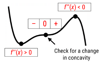
Step ❹ : Only find points of inflection if required to by the question.
- Solve \(f''(x) = 0\) to find x-intercepts of possible points of inflection.
- Test possible POI by substituting the x-coordinates of points either side of the possible POI into \(f''(x) \). A change of sign indicates a change in concavity and hence a POI.
Step ❺ : If possible, find x-intercept(s) (sub y=0 and solve) and y-intercept (sub x = 0 and evaluate).
Step ❻ : Examine domain and range for discontinuities (denominator = 0) or asymptotes (consider limits).
Step ❼ : Find the range of endpoints if given an interval to sketch in.
Step ❽ : Use the information from the previous steps to sketch a graph of the function.
Practice
Locate and determine the nature of any stationary points on the following functions.